9  Enrichment Spiralize

Note

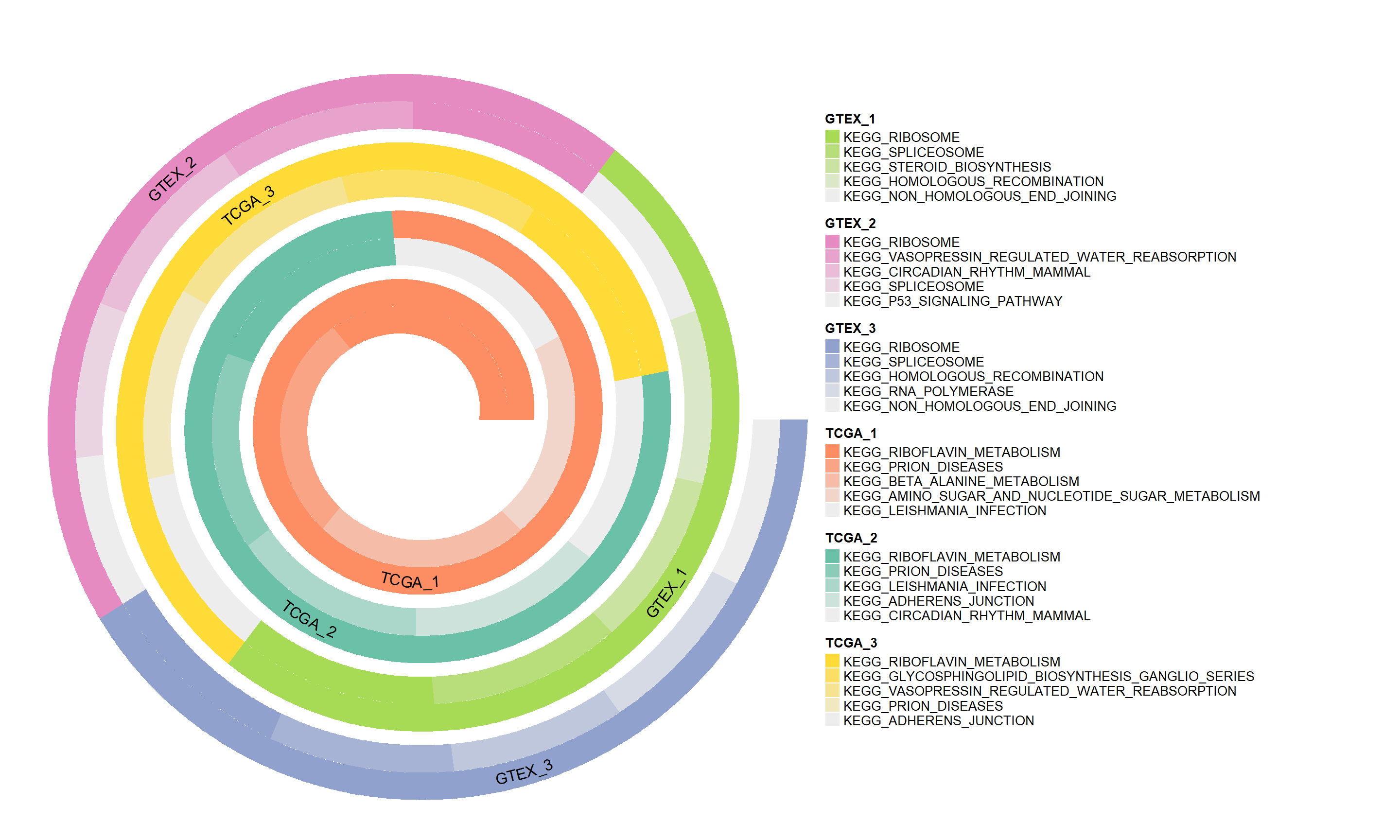
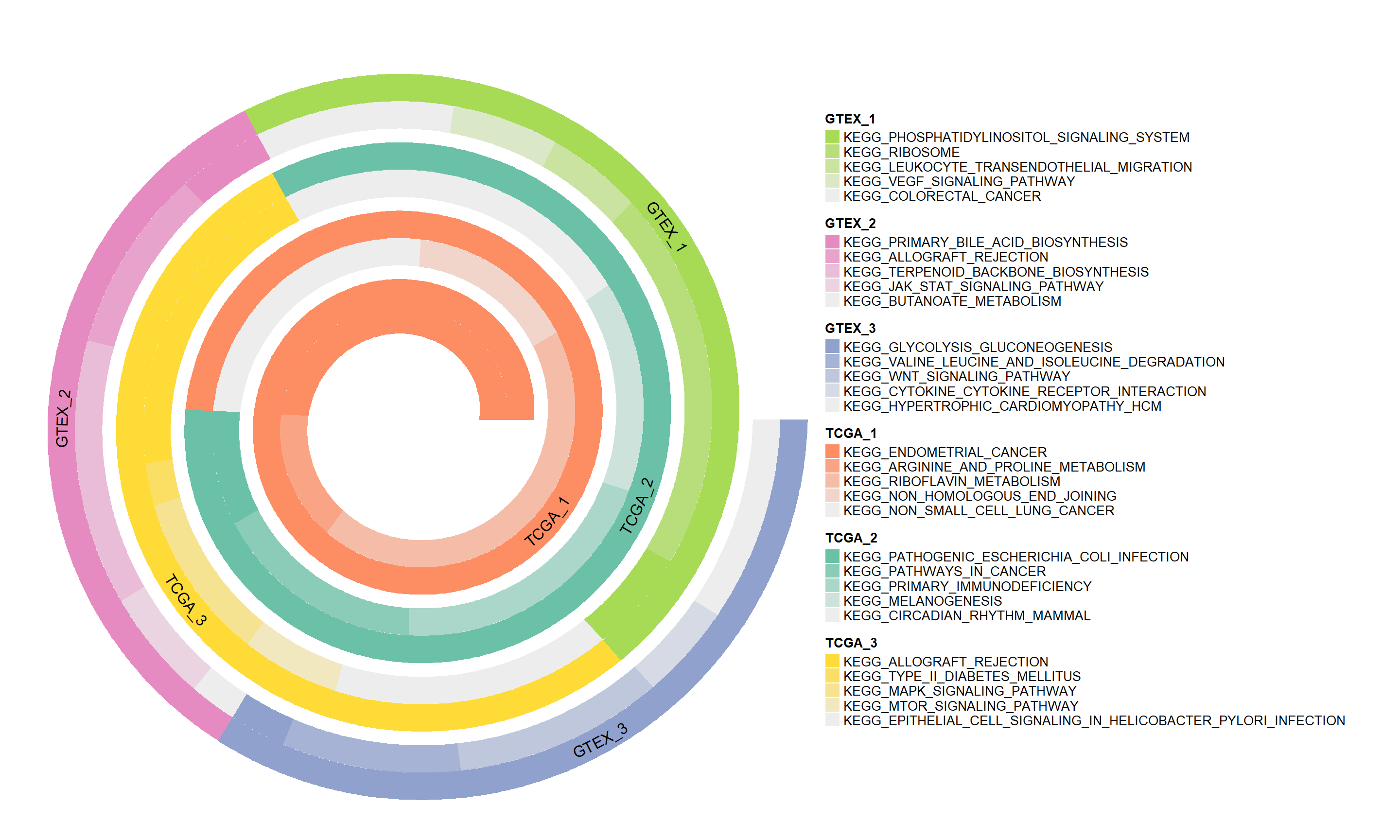
The spiral plots generated by this module provide an intuitive visual display, depicting the expression changes in different biological pathways across samples through gradient colors and spatial arrangement. This visualization method helps to more clearly identify and compare the activity differences in key pathways, thereby deepening the understanding of physiological mechanisms.

library(TransProR)
library(org.Hs.eg.db)
library(clusterProfiler)
library(tidyr)
library(dplyr)
library(ggplot2)
library(GSVA)
library(msigdbr)
library(scales)

9.1 load data

tumor <- readRDS("../test_TransProR/generated_data1/removebatch_SKCM_Skin_TCGA_exp_tumor.rds")
normal <- readRDS('../test_TransProR/generated_data1/removebatch_SKCM_Skin_Normal_TCGA_GTEX_count.rds')
# Merge the datasets, ensuring both have genes as row names
all_count_exp <- merge(tumor, normal, by = "row.names")
all_count_exp <- tibble::column_to_rownames(all_count_exp, var = "Row.names")  # Set the row names

# Drawing data
# all_count_exp <- log_transform(all_count_exp)
DEG_deseq2 <- readRDS('../test_TransProR/Select DEGs/DEG_deseq2.Rdata')
#head(all_count_exp, 1)
head(DEG_deseq2, 5)
          baseMean log2FoldChange      lfcSE      stat pvalue padj change
A1BG      134.6084      -2.549682 0.05677219 -44.91075      0    0   down
A2M     30208.9912       3.251168 0.08394645  38.72907      0    0     up
AADACL2   801.4538      -8.229956 0.18969649 -43.38486      0    0   down
AARS2    1153.5493       1.624753 0.03283522  49.48202      0    0 stable
AARSD1    567.8672      -2.082289 0.02275703 -91.50088      0    0 stable

9.2 Convert from SYMBOL to ENTREZID

# Convert from SYMBOL to ENTREZID for convenient enrichment analysis later. It's crucial to do this now as a direct conversion may result in a reduced set of genes due to non-one-to-one correspondence.

# DEG_deseq2
# Retrieve gene list
gene <- rownames(DEG_deseq2)
# Perform conversion
gene = bitr(gene, fromType="SYMBOL", toType="ENTREZID", OrgDb="org.Hs.eg.db")
'select()' returned 1:many mapping between keys and columns
Warning in bitr(gene, fromType = "SYMBOL", toType = "ENTREZID", OrgDb =
"org.Hs.eg.db"): 43.37% of input gene IDs are fail to map...
# Remove duplicates and merge
gene <- dplyr::distinct(gene, SYMBOL, .keep_all=TRUE)
# Extract the SYMBOL column as a vector from the first dataset
symbols_vector <- gene$SYMBOL
# Use the SYMBOL column to filter corresponding rows from the second dataset by row names
DEG_deseq2 <- DEG_deseq2[rownames(DEG_deseq2) %in% symbols_vector, ]
head(DEG_deseq2, 5)
          baseMean log2FoldChange      lfcSE      stat pvalue padj change
A1BG      134.6084      -2.549682 0.05677219 -44.91075      0    0   down
A2M     30208.9912       3.251168 0.08394645  38.72907      0    0     up
AADACL2   801.4538      -8.229956 0.18969649 -43.38486      0    0   down
AARS2    1153.5493       1.624753 0.03283522  49.48202      0    0 stable
AARSD1    567.8672      -2.082289 0.02275703 -91.50088      0    0 stable
Diff_deseq2 <- filter_diff_genes(
  DEG_deseq2, 
  p_val_col = "pvalue", 
  log_fc_col = "log2FoldChange",
  p_val_threshold = 0.05, 
  log_fc_threshold = 3
)
# First, obtain a list of gene names from the row names of the first dataset
gene_names <- rownames(Diff_deseq2)
# Find the matching rows in the second dataframe
matched_rows <- all_count_exp[gene_names, ]
# Calculate the mean for each row
averages <- rowMeans(matched_rows, na.rm = TRUE)
# Append the averages as a new column to the first dataframe
Diff_deseq2$average <- averages
Diff_deseq2$ID <- rownames(Diff_deseq2)
Diff_deseq2$changetype <- ifelse(Diff_deseq2$change == 'up', 1, -1)
# Define a small threshold value
small_value <- .Machine$double.xmin
# Before calculating -log10, replace zeroes with the small threshold value and assign it to a new column
Diff_deseq2$log_pvalue <- ifelse(Diff_deseq2$pvalue == 0, -log10(small_value), -log10(Diff_deseq2$pvalue))
# Extract the expression data corresponding to the differentially expressed genes
heatdata_deseq2 <- all_count_exp[rownames(Diff_deseq2), ]

set.seed(123)
# Preparing heatdata for visualization
HeatdataDeseq2 <- TransProR::process_heatdata(heatdata_deseq2, 
                                              selection = 2, 
                                              custom_names = NULL, 
                                              num_names_per_group = 3, 
                                              prefix_length = 4)
HeatdataDeseq2 <- as.matrix(HeatdataDeseq2)
## Using the msigdbr package to download and prepare for GSVA analysis with KEGG and GO gene sets
## KEGG
KEGG_df_all <- msigdbr(species = "Homo sapiens", # Homo sapiens or Mus musculus
                        category = "C2",
                        subcategory = "CP:KEGG") 
KEGG_df <- dplyr::select(KEGG_df_all, gs_name, gs_exact_source, gene_symbol)
kegg_list <- split(KEGG_df$gene_symbol, KEGG_df$gs_name) # Grouping gene symbols by gs_name
head(kegg_list)
$KEGG_ABC_TRANSPORTERS
 [1] "ABCA1"  "ABCA10" "ABCA12" "ABCA13" "ABCA2"  "ABCA3"  "ABCA4"  "ABCA5" 
 [9] "ABCA6"  "ABCA7"  "ABCA8"  "ABCA9"  "ABCB1"  "ABCB10" "ABCB11" "ABCB11"
[17] "ABCB4"  "ABCB5"  "ABCB6"  "ABCB7"  "ABCB8"  "ABCB9"  "ABCC1"  "ABCC1" 
[25] "ABCC10" "ABCC11" "ABCC12" "ABCC2"  "ABCC3"  "ABCC4"  "ABCC5"  "ABCC6" 
[33] "ABCC6"  "ABCC8"  "ABCC9"  "ABCD1"  "ABCD2"  "ABCD3"  "ABCD4"  "ABCG1" 
[41] "ABCG2"  "ABCG4"  "ABCG5"  "ABCG8"  "CFTR"   "TAP1"   "TAP1"   "TAP1"  
[49] "TAP1"   "TAP1"   "TAP1"   "TAP1"   "TAP1"   "TAP2"   "TAP2"   "TAP2"  
[57] "TAP2"   "TAP2"   "TAP2"   "TAP2"   "TAP2"  

$KEGG_ACUTE_MYELOID_LEUKEMIA
 [1] "AKT1"     "AKT2"     "AKT3"     "AKT3"     "ARAF"     "BAD"     
 [7] "BRAF"     "CCNA1"    "CCND1"    "CEBPA"    "CHUK"     "EIF4EBP1"
[13] "FLT3"     "GRB2"     "HRAS"     "HRAS"     "IKBKB"    "IKBKG"   
[19] "JUP"      "KIT"      "KRAS"     "LEF1"     "MAP2K1"   "MAP2K2"  
[25] "MAPK1"    "MAPK3"    "MTOR"     "MYC"      "NFKB1"    "NRAS"    
[31] "PIK3CA"   "PIK3CB"   "PIK3CD"   "PIK3CG"   "PIK3R1"   "PIK3R2"  
[37] "PIK3R3"   "PIK3R5"   "PIM1"     "PIM2"     "PML"      "PPARD"   
[43] "RAF1"     "RARA"     "RELA"     "RPS6KB1"  "RPS6KB2"  "RUNX1"   
[49] "RUNX1T1"  "SOS1"     "SOS2"     "SPI1"     "STAT3"    "STAT5A"  
[55] "STAT5B"   "TCF7"     "TCF7L1"   "TCF7L2"   "ZBTB16"  

$KEGG_ADHERENS_JUNCTION
 [1] "ACP1"    "ACTB"    "ACTG1"   "ACTN1"   "ACTN2"   "ACTN3"   "ACTN4"  
 [8] "ACTN4"   "AFDN"    "BAIAP2"  "CDC42"   "CDH1"    "CREBBP"  "CSNK2A1"
[15] "CSNK2A2" "CSNK2B"  "CSNK2B"  "CSNK2B"  "CSNK2B"  "CSNK2B"  "CSNK2B" 
[22] "CSNK2B"  "CSNK2B"  "CTNNA1"  "CTNNA2"  "CTNNA3"  "CTNNB1"  "CTNND1" 
[29] "EGFR"    "EP300"   "ERBB2"   "FARP2"   "FER"     "FGFR1"   "FYN"    
[36] "IGF1R"   "INSR"    "IQGAP1"  "LEF1"    "LMO7"    "MAP3K7"  "MAPK1"  
[43] "MAPK3"   "MET"     "NECTIN1" "NECTIN2" "NECTIN3" "NECTIN4" "NLK"    
[50] "PARD3"   "PTPN1"   "PTPN6"   "PTPRB"   "PTPRF"   "PTPRJ"   "PTPRM"  
[57] "RAC1"    "RAC2"    "RAC3"    "RHOA"    "SMAD2"   "SMAD3"   "SMAD4"  
[64] "SNAI1"   "SNAI2"   "SORBS1"  "SRC"     "SSX2IP"  "TCF7"    "TCF7L1" 
[71] "TCF7L2"  "TGFBR1"  "TGFBR2"  "TJP1"    "TJP1"    "VCL"     "WAS"    
[78] "WASF1"   "WASF2"   "WASF3"   "WASL"    "YES1"   

$KEGG_ADIPOCYTOKINE_SIGNALING_PATHWAY
 [1] "ACACB"    "ACSL1"    "ACSL3"    "ACSL4"    "ACSL5"    "ACSL6"   
 [7] "ADIPOQ"   "ADIPOR1"  "ADIPOR2"  "ADIPOR2"  "AGRP"     "AKT1"    
[13] "AKT2"     "AKT3"     "AKT3"     "CAMKK1"   "CAMKK2"   "CD36"    
[19] "CHUK"     "CPT1A"    "CPT1B"    "CPT1C"    "G6PC1"    "G6PC2"   
[25] "G6PC2"    "IKBKB"    "IKBKG"    "IRS1"     "IRS2"     "IRS4"    
[31] "JAK2"     "LEP"      "LEPR"     "MAPK10"   "MAPK8"    "MAPK9"   
[37] "MTOR"     "NFKB1"    "NFKBIA"   "NFKBIB"   "NFKBIB"   "NFKBIE"  
[43] "NPY"      "PCK1"     "PCK2"     "PCK2"     "POMC"     "PPARA"   
[49] "PPARGC1A" "PRKAA1"   "PRKAA2"   "PRKAB1"   "PRKAB2"   "PRKAG1"  
[55] "PRKAG2"   "PRKAG3"   "PRKCQ"    "PTPN11"   "RELA"     "RXRA"    
[61] "RXRB"     "RXRB"     "RXRB"     "RXRB"     "RXRB"     "RXRB"    
[67] "RXRG"     "SLC2A1"   "SLC2A4"   "SLC2A4"   "SOCS3"    "STAT3"   
[73] "STK11"    "TNF"      "TNF"      "TNF"      "TNF"      "TNF"     
[79] "TNF"      "TNF"      "TNF"      "TNFRSF1A" "TNFRSF1B" "TRADD"   
[85] "TRAF2"   

$KEGG_ALANINE_ASPARTATE_AND_GLUTAMATE_METABOLISM
 [1] "ABAT"    "ACY3"    "ADSL"    "ADSS1"   "ADSS2"   "AGXT"    "AGXT2"  
 [8] "ALDH4A1" "ALDH5A1" "ASL"     "ASNS"    "ASPA"    "ASS1"    "CAD"    
[15] "CPS1"    "DDO"     "GAD1"    "GAD2"    "GFPT1"   "GFPT2"   "GLS"    
[22] "GLS2"    "GLUD1"   "GLUD2"   "GLUD2"   "GLUL"    "GOT1"    "GOT2"   
[29] "GPT"     "GPT2"    "IL4I1"   "NIT2"    "PPAT"   

$KEGG_ALDOSTERONE_REGULATED_SODIUM_REABSORPTION
 [1] "ATP1A1"   "ATP1A2"   "ATP1A3"   "ATP1A4"   "ATP1B1"   "ATP1B2"  
 [7] "ATP1B3"   "ATP1B4"   "FXYD2"    "FXYD4"    "HSD11B1"  "HSD11B2" 
[13] "IGF1"     "INS"      "INSR"     "IRS1"     "IRS2"     "IRS4"    
[19] "KCNJ1"    "KRAS"     "MAPK1"    "MAPK3"    "NEDD4L"   "NR3C2"   
[25] "PDPK1"    "PIK3CA"   "PIK3CB"   "PIK3CD"   "PIK3CG"   "PIK3R1"  
[31] "PIK3R2"   "PIK3R3"   "PIK3R5"   "PRKCA"    "PRKCB"    "PRKCG"   
[37] "SCNN1A"   "SCNN1B"   "SCNN1G"   "SFN"      "SGK1"     "SLC9A3R2"
## GO
GO_df_all <- msigdbr(species = "Homo sapiens",
                      category = "C5")  
GO_df <- dplyr::select(GO_df_all, gs_name, gene_symbol, gs_exact_source, gs_subcat)
GO_df <- GO_df[GO_df$gs_subcat != "HPO",]
go_list <- split(GO_df$gene_symbol, GO_df$gs_name) # Grouping gene symbols by gs_name
head(go_list)
$GOBP_10_FORMYLTETRAHYDROFOLATE_METABOLIC_PROCESS
[1] "AASDHPPT" "ALDH1L1"  "ALDH1L2"  "MTHFD1"   "MTHFD1L"  "MTHFD2L" 

$GOBP_2_OXOGLUTARATE_METABOLIC_PROCESS
 [1] "AADAT"  "ADHFE1" "D2HGDH" "DLST"   "GOT1"   "GOT2"   "GPT2"   "IDH1"  
 [9] "IDH2"   "IDH3B"  "KYAT3"  "L2HGDH" "MRPS36" "MRPS36" "OGDH"   "OGDHL" 
[17] "PHYH"   "TAT"   

$GOBP_2FE_2S_CLUSTER_ASSEMBLY
[1] "BOLA2"  "BOLA2B" "GLRX3"  "GLRX5"  "HSCB"   "NFS1"  

$GOBP_3_PHOSPHOADENOSINE_5_PHOSPHOSULFATE_BIOSYNTHETIC_PROCESS
[1] "PAPSS1"  "PAPSS2"  "SLC26A1" "SLC26A2" "SLC35B2" "SLC35B3"

$GOBP_3_PHOSPHOADENOSINE_5_PHOSPHOSULFATE_METABOLIC_PROCESS
 [1] "ABHD14B" "BPNT1"   "ENPP1"   "PAPSS1"  "PAPSS2"  "SLC26A1" "SLC26A2"
 [8] "SLC35B2" "SLC35B3" "SULT1A1" "SULT1A2" "SULT1A3" "SULT1A4" "SULT1B1"
[15] "SULT1C3" "SULT1C4" "SULT1E1" "SULT2A1" "SULT2B1" "TPST1"   "TPST2"  

$GOBP_3_UTR_MEDIATED_MRNA_DESTABILIZATION
 [1] "CPEB3"   "DHX36"   "DHX36"   "DND1"    "DND1"    "HNRNPD"  "KHSRP"  
 [8] "MOV10"   "PLEKHN1" "RBM24"   "RC3H1"   "TARDBP"  "TRIM71"  "UPF1"   
[15] "ZC3H12A" "ZC3H12D" "ZFP36"   "ZFP36L1" "ZFP36L2"
#write.csv(gsva_mat, "gsva_go_matrix.csv")

ssgsea_kegg <- gsva(expr = HeatdataDeseq2, 
                    gset.idx.list = kegg_list, 
                    kcdf = "Poisson", #"Gaussian" for logCPM, logRPKM, logTPM, "Poisson" for counts
                    method = "ssgsea",
                    verbose = TRUE
                    #parallel.sz = parallel::detectCores() # Utilize all available cores
)
Warning: Calling gsva(expr=., gset.idx.list=., method=., ...) is deprecated;
use a method-specific parameter object (see '?gsva').
Warning in .filterFeatures(expr, method): 37 genes with constant expression
values throughout the samples.
Warning in .gsva(expr, mapped.gset.idx.list, method, kcdf, rnaseq, abs.ranking,
: Some gene sets have size one. Consider setting 'min.sz > 1'.
Estimating ssGSEA scores for 171 gene sets.
[1] "Calculating ranks..."
[1] "Calculating absolute values from ranks..."

  |                                                                            
  |                                                                      |   0%
  |                                                                            
  |============                                                          |  17%
  |                                                                            
  |=======================                                               |  33%
  |                                                                            
  |===================================                                   |  50%
  |                                                                            
  |===============================================                       |  67%
  |                                                                            
  |==========================================================            |  83%
  |                                                                            
  |======================================================================| 100%

[1] "Normalizing..."
ssgsea_kegg <- as.data.frame(ssgsea_kegg)

9.3 set color

nTop = 5
results1 <- extract_ntop_pathways(ssgsea_kegg = ssgsea_kegg, nTop = nTop)
results2 <- extract_positive_pathways(ssgsea_kegg, max_paths_per_sample = 5)
# Set the required number of transition colors

number_of_colors <- nTop

# Define start and end colors
start_color1 <- "#fd8d63"  
end_color1 <- "#ededed"    
# Use colorRampPalette to generate color transitions
color_palette1 <- colorRampPalette(c(start_color1, end_color1))
interpolated_colors1 <- color_palette1(number_of_colors)

start_color2 <- "#673ab7"  
end_color2 <- "#d1c4e9"    
color_palette2 <- colorRampPalette(c(start_color2, end_color2))
interpolated_colors2 <- color_palette2(number_of_colors)

start_color3 <- "#6ac1a7"  
end_color3 <- "#ededed"    
color_palette3 <- colorRampPalette(c(start_color3, end_color3))
interpolated_colors3 <- color_palette3(number_of_colors)

start_color4 <- "#2196f3"  
end_color4 <- "#bbdefb"    
color_palette4 <- colorRampPalette(c(start_color4, end_color4))
interpolated_colors4 <- color_palette4(number_of_colors)

start_color5 <- "#ffdb37"  
end_color5 <- "#ededed"    
color_palette5 <- colorRampPalette(c(start_color5, end_color5))
interpolated_colors5 <- color_palette5(number_of_colors)

start_color6 <- "#00bcd4"  
end_color6 <- "#b2ebf2"    
color_palette6 <- colorRampPalette(c(start_color6, end_color6))
interpolated_colors6 <- color_palette6(number_of_colors)

start_color7 <- "#a7da55"  
end_color7 <- "#ededed"    
color_palette7 <- colorRampPalette(c(start_color7, end_color7))
interpolated_colors7 <- color_palette7(number_of_colors)

start_color8 <- "#43a047"  
end_color8 <- "#c8e6c9"    
color_palette8 <- colorRampPalette(c(start_color8, end_color8))
interpolated_colors8 <- color_palette8(number_of_colors)

start_color9 <- "#e68bc1"  
end_color9 <- "#ededed"    
color_palette9 <- colorRampPalette(c(start_color9, end_color9))
interpolated_colors9 <- color_palette9(number_of_colors)

start_color10 <- "#cddc39"  
end_color10 <- "#f0f4c3"    
color_palette10 <- colorRampPalette(c(start_color10, end_color10))
interpolated_colors10 <- color_palette10(number_of_colors)

start_color11 <- "#8fa1cc"  
end_color11 <- "#ededed"    
color_palette11 <- colorRampPalette(c(start_color11, end_color11))
interpolated_colors11 <- color_palette11(number_of_colors)

start_color12 <- "#ff8f00"  
end_color12 <- "#ffecb3"    
color_palette12 <- colorRampPalette(c(start_color12, end_color12))
interpolated_colors12 <- color_palette12(number_of_colors)

# Print the resulting colors
Pathwaycolor2 <- c(interpolated_colors1, interpolated_colors3, interpolated_colors5, interpolated_colors7, interpolated_colors9, interpolated_colors11)
print(Pathwaycolor2)
 [1] "#FD8D63" "#F9A585" "#F5BDA8" "#F1D5CA" "#EDEDED" "#6AC1A7" "#8ACCB8"
 [8] "#ABD7CA" "#CCE2DB" "#EDEDED" "#FFDB37" "#FADF64" "#F6E392" "#F1E8BF"
[15] "#EDEDED" "#A7DA55" "#B8DE7B" "#CAE3A1" "#DBE8C7" "#EDEDED" "#E68BC1"
[22] "#E7A3CC" "#E9BCD7" "#EBD4E2" "#EDEDED" "#8FA1CC" "#A6B3D4" "#BEC7DC"
[29] "#D5DAE4" "#EDEDED"
Samplecolor2 <- c(start_color1, start_color3, start_color5, start_color7, start_color9, start_color11)
print(Samplecolor2)
[1] "#fd8d63" "#6ac1a7" "#ffdb37" "#a7da55" "#e68bc1" "#8fa1cc"
results1$PathwayColor <- Pathwaycolor2
results2$PathwayColor <- Pathwaycolor2
# Create a color mapping for the Sample column
Sample_colors2 <- setNames(Samplecolor2, unique(results1$Sample))
Sample_colors2 <- setNames(Samplecolor2, unique(results2$Sample))
# Add SampleColor column to the DataFrame
results1$SampleColor <- Sample_colors2[results1$Sample]
results2$SampleColor <- Sample_colors2[results2$Sample]
# View the results
print(head(results1))
                                           Pathway Sample     Value
1                       KEGG_RIBOFLAVIN_METABOLISM TCGA_1 0.5417180
2                              KEGG_PRION_DISEASES TCGA_1 0.5324760
3                     KEGG_BETA_ALANINE_METABOLISM TCGA_1 0.5187272
4 KEGG_AMINO_SUGAR_AND_NUCLEOTIDE_SUGAR_METABOLISM TCGA_1 0.5169535
5                        KEGG_LEISHMANIA_INFECTION TCGA_1 0.5003448
6                       KEGG_RIBOFLAVIN_METABOLISM TCGA_2 0.5345860
  PathwayColor SampleColor
1      #FD8D63     #fd8d63
2      #F9A585     #fd8d63
3      #F5BDA8     #fd8d63
4      #F1D5CA     #fd8d63
5      #EDEDED     #fd8d63
6      #6AC1A7     #6ac1a7
print(head(results2))
                                     Pathway Sample     Value PathwayColor
1                    KEGG_ENDOMETRIAL_CANCER TCGA_1 0.4091193      #FD8D63
2       KEGG_ARGININE_AND_PROLINE_METABOLISM TCGA_1 0.1608353      #F9A585
3                 KEGG_RIBOFLAVIN_METABOLISM TCGA_1 0.5417180      #F5BDA8
4            KEGG_NON_HOMOLOGOUS_END_JOINING TCGA_1 0.2218331      #F1D5CA
5            KEGG_NON_SMALL_CELL_LUNG_CANCER TCGA_1 0.3934194      #EDEDED
6 KEGG_PATHOGENIC_ESCHERICHIA_COLI_INFECTION TCGA_2 0.1543440      #6AC1A7
  SampleColor
1     #fd8d63
2     #fd8d63
3     #fd8d63
4     #fd8d63
5     #fd8d63
6     #6ac1a7

9.4 Sort

enrichment_spiral_plots(results1)

9.5 Random

enrichment_spiral_plots(results2)

9.6 Reference

  • spiralize:

Zuguang Gu, et al., spiralize: an R package for Visualizing Data on Spirals, Bioinformatics, 2021.

  • ComplexHeatmap:

Complex heatmaps reveal patterns and correlations in multidimensional genomic data

Complex heatmap visualization

  • ggplot2:

github:ggplot2

An implementation of the Grammar of Graphics in R